• View
• Edit
• History
• Print

Define The Compression Direction

Data coverage in axial and radial experiments

Explaining data coverage takes a lot of figures, so I moved it into separate sections:

• Using pole figures to represent directions in space
• Data coverage in axial diffraction experiments
• Data coverage in radial diffraction experiments

In summary, the data coverage from one diffraction ring should look like the figure below. Direction of compression is in the center, data coverage is in red, blue indicate values for the angle alpha and beta, and brown is used to locate points corresponding to specific azimuth on the imaging plate.

Figure 1: data coverage in axial geometry	Figure 2: data coverage in the radial geometry

In the axial geometry, all orientations on a diffraction ring are located at the same distance from the compression direction, beta = 90-theta, where theta is the diffraction angle. If one make the assumption of an axial symmetry around the compression direction, they all probe the same orientation.

In the radial geometry, various orientations on the diffraction ring probe different distances of the compression direction. If one assumes an axial symmetry around the compression direction, we probe the all space of orientations.

Finding out orientation coverage in Maud

When running MAUD, they can be issues with the orientations of your datafiles. Things can be rotated within MAUD, and experiments are not always performed in the same geometry.

To find out your coverage, the easiest way I know off is to to use the texture functions. Open the Graphic -> Texture plot menu item. You'll have a window with various plotting options. Select one diffraction from a material, a plot the Pole figure coverage. In radial geometry, it should look like the figure below.

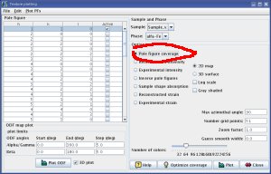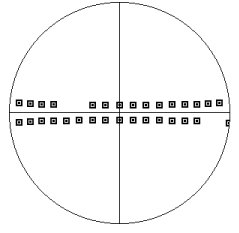Figure 3: Plotting pole figure data coverage	Figure 4: Example of data coverage for a radial diffraction experiment

If you're dealing with a radial diffraction experiment and your coverage looks like Figure 1, something is wrong with your orientations. It should look like Figure 4.

Locating the compression direction

The next step is to locate your compression direction. It should be at the center of the pole figure, otherwise, things will not work properly:

• the stress model will be wrong,
• applying cylindrical symmetry for texture refinement will fail.

In order to check that your compression direction is ok,

• open the dataset window,
• select a datafile that you know is on the compression direction,
• disable it (there is a little checkbox to do this, near the dialog below the filelist),
• replot the pole figure coverage,
• one of the squares in the figure (like the one in Figure 4) should be gone,
• make sure that the square that disappeared was near the center of the pole figure.

If the square that disappeared was on the outside rim, something is wrong with your orientations: the data for the compression direction does not point to the center of pole figure.

Fixing things out

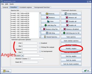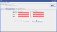Figure 5: Playing with orientations in the dataset window	Figure 6: Playing with orientations in the sample window

There are two ways to bring you data into the proper orientation

• in the dataset window (Figure 5),
• in the Sample position tab of the Sample window (Figure 6).

In the dataset window, eta angles are azimuth on the image plate. The other angles define the orientation of the dataset relative to the sample.

The sample position tab allows you to rotate the whole sample for the analysis.

I do not have a good way to do this: just find the angles that will bring you the orientation you want. There are multiple solutions and it depends on your experimental setup...